Translate this page into:
How to Perform Discriminant Analysis in Medical Research? Explained with Illustrations

Address for correspondence: Deepak Dhamnetiya, MD, Assistant Professor, Department of Community Medicine, Dr Baba Saheb Ambedkar Medical College & Hospital, Sector-6, Rohini, New Delhi 110085, India (e-mail: drdeepakdhamnetiya@gmail.com).
This article was originally published by Thieme Medical and Scientific Publishers Pvt. Ltd. and was migrated to Scientific Scholar after the change of Publisher.
Abstract
Discriminant function analysis is the statistical analysis used to analyze data when the dependent variable or outcome is categorical and independent variable or predictor variable is parametric. It is a parametric technique to determine which weightings of quantitative variables or predictors best discriminates between two or more than two categories of dependent variables and does so better than chance. Discriminant analysis is used to find out the accuracy of a given classification system in predicting the sample into a particular group. Discriminant analysis includes the development of discriminant functions for each sample and deriving a cutoff score that is used for classifying the samples into different groups. Discriminant function analysis is a statistical analysis used to find out the accuracy of a given classification system or predictor variables. This article explains the basic assumptions, uses, and necessary requirements of discriminant analysis with a real-life clinical example. Whenever a new classification system is introduced, discriminant function analysis can be used to find out the accuracy with which the classification is able to differentiate a particular sample into different groups. Thus, it is a very useful tool in medical research where classification is required.
Keywords
discriminant analysis
discriminant equation
canonical discriminant functions
centroid

The Problem of Classification of Observations
The problem of classification arises when an investigator tries to classify a number of individuals into two or more categories or tries to decide in which category these individuals should be kept depending on a number of measurements available on each of those individuals. The direct identification of these individuals with their respective categories is impossible and hence this is considered as a problem of constructing a suitable “statistical decision function” assuming that these individuals have come from a finite number of different populations that can be characterized by different probability distributions and the question simplifies to “given an individual with a number of measurements on different variables, which population did the person come from?” In the next section, we have discussed a statistical technique of classification, called “discriminant analysis (DA)”.
Discriminant Analysis
DA is a parametric technique to determine which weightings of quantitative variables or predictors best discriminates between two or more than two categories of dependent variables and does so better than chance.[1]
In other words, DA is the most popular statistical technique to classify individuals or observations into nonoverlapping groups, based on scores derived from a suitable “statistical decision function” constructed from one or more continuous predictor variables.
For example, if a doctor wishes to identify patients with high, moderate, and low risk of developing heart complications like stroke, he or she can perform a DA to classify patients at different risk groups for stroke. Such a method enables the doctor to classify patients into high-moderate-low-risk groups, based on personal attributes (e.g., high-density lipoprotein [HDL] level, low-density lipoprotein [LDL] level, cholesterol level, body mass index) and/or lifestyle behaviors (e.g., hours of exercise or physical activities per week, smoking status like number of cigarettes per day).
Preliminary Considerations of DA
DA undertakes the same task as multiple linear regression by predicting an outcome on the basis of given set of predictors. However, multiple linear regression is limited to cases where the dependent variable on the Y axis is an interval variable so that the combination of predictors will, through the regression equation, produce estimated mean population numerical Y values for given values of weighted combinations of X values. The problem arises when the dependent variable is categorical in nature, like status/stages of a particular disease and migrant/nonmigrant status. Together with that, it is desired to minimize the probability of misclassification as well.
Purposes of Discriminant Analysis
While investigating the differences between the groups or categories, the necessary step is to identify the attributes with most contributions to maximum separability between known groups or categories in order to classify a given observation in to one of the groups. For that purpose, DA successively identifies the linear combination of attributes known as canonical discriminant functions (equations) that contribute maximally to group separation. Predictive DA addresses the question of how to assign new cases to groups. The DA function produces scores for individuals on the predictor variables to predict the category to which that individual belongs. DA is considered to determine the most parsimonious way to distinguish between groups. Statistical significance tests using chi-square enable the investigator to see how well the function separates the groups. Last but not the least, DA also enables the investigator to test theory whether cases are classified as predicted.
Key Assumptions of DA: The following assumptions are necessary for DA:
The observations are a random sample from different populations characterized by different probability distributions.
Each predictor variable is assumed to be normally distributed.
Each of the allocations for the dependent categories in the initial classification is correctly classified and groups or categories should be defined before collecting the data.
There must be at least two groups or categories, with each case belonging to only one group so that the groups are mutually exclusive and collectively exhaustive (all cases can be placed in a group).
The attribute(s) used to separate the groups should discriminate quite clearly between the groups so that group or category overlap is clearly nonexistent or minimal.
Group sizes of the dependent should not be grossly different and should be at least five times the number of independent variables.[2]
Depending on the number of categories and the method of constructing the discriminant function, there are several types of DA, such as linear, multiple, and quadratic DA (QDA). In the next sections, we have discussed the linear DA (LDA).
DA Linear Equation
DA involves the determination of a linear equation like regression that will predict which group the case belongs to. The form of the equation or function is:
D = v1X1 + v2X2 + v3X3 + ………………...+ viXp + a
Where D = discriminate function
vi = The discriminant coefficient or weight for that variable
Xi = Respondent's score for the ith variable
a = constant
p = the number of predictor variables
The v's are unstandardized discriminant coefficients analogous to the b's in the regression equation (Y= b1X1 + b2X2 + b3X3 + ………………... + biXp + a). These v's maximize the distance between the means of the criterion (dependent) variable. Standardized discriminant coefficients can also be used like beta weight in regression. Good predictors tend to have large weights. Now this function should maximize the distance between the categories, that is, come up with an equation that has strong discriminatory power between groups, or to maximize the standardized squared distance between the two populations. After using an existing set of data to calculate the discriminant function and classify cases, any new cases can then be classified. The number of discriminant functions is one less the number of groups. There is only one function for the basic two group DA.
Sample Size for DA
In DA, the rule for determining the appropriate sample size largely depends on the complexity of the subject of study and the environment of the study population. The sample selected should be a proper representative of the study population as well as the environment. Fewer sample observations are needed to properly represent a homogeneous environment, and they will be sufficient to uncover any patterns that exist. Beyond this, there definitely are some general rules to follow, together with some specific rules proposed by various authors to tackle specific situations.
General Rules
As in case of all eigen analysis problems, the minimum sample observations should be at least as many as the total variables. In case of DA, however, there must be at least two more sample observations than the number of variables and there should be at least two observations per group as well. Together with this, enough sample observations for each group should be taken to ensure accurate and more precise estimation of means and dispersions for groups.
One conventional way of doing this is sequential sampling until the mean and variance of the parameter estimates (e.g., eigenvalues, canonical coefficients) stabilize. From the acquired data, the stability of the results can always be assessed using a proper resampling technique, and the results then can be utilized to determine the sample size needed to estimate the parameters with the desired level of precision in future studies.
Specific Rules
Apart from the general rules discussed earlier, there are some specific rules owing to different specific situations. Such rules are suggested by different authors. These rules are based on P and G (P = number of discriminating variables, and G = number of groups):
Rule A N ≥ 20 + 3P[3]
Rule B If P ≤ 4,N ≥ 25G
If P > 4, N ≥ [25 + 12(P - 4)]G[4]
Rule C For each group, N ≥ 3P[5]
Rule C is considered as the best guide for determining the appropriate sample size as it is derived from extensive simulation results. Though in practice, group sample sizes and number of groups are often fixed. In such a situation, and when full data set does not meet sample size requirements, then one should roughly calculate the number of variables to be included in the analysis given the fixed number of groups and group sample sizes. If the investigator feels the need to reduce number of variables, then the conventional way is to remove those variables with less significance or having less ability to discriminate among group in their order of relevance.
The alternative technique is that the variables can be divided into two or more groups of related variables, and separate DAs are done on each group. Alternatively, stepwise discrimination procedures can be utilized to select the best set of discriminating variables from each subset of variables and then the investigator needs to combine them into one subsequent analysis. In critical situations when the investigator is forced to work with sample sizes smaller than the quantity calculated by using Rule C, the stability of the parameter estimates should be evaluated by utilizing a suitable resampling method and the results thus obtained should be interpreted with caution.
DA based on number of groups: Depending upon the number of groups of dependent variable, the LDA is of two types:
Two-group DA
Multiple group DA
Two-Group DA
A common research problem involves classifying observations into one of two groups, based on two or more continuous predictor variables.
The form of the equation or function for two-group DA is:
D = v1X1 + v2X2 + a
The dependent variable is a dichotomous, categorical variable (i.e., a categorical variable that can take only two values).
The dependent variable is expressed as a dummy variable (having values of 0 or 1).
Observations are assigned to groups, based on whether the predicted score is closer to 0 or to 1.
The regression equation is called the discriminant function.
The efficacy of the discriminant function is measured by the proportion of correct classification.
Multiple Group Discriminant Analysis
Regression can also be used with more than two classification groups, but the analysis is more complicated. When there are more than two groups, there are also more than one discriminant functions.
For example, suppose you wanted to classify disease into one of the three disease status—mild, moderate, or severe. Using two-group DA, you might:
Define one discriminant function to classify disease status as mild or nonmild cases.
Define a second discriminant function to classify nonmild case as moderate case or severe case.
The maximum number of discriminant functions will equal the number of predictor variables or the number of group categories minus one—whichever is smaller. With multiple DA, the goal is to define discriminant functions that maximize differences between groups and minimize differences within groups.
How to Perform DA?
In this section, we illustrate how to perform DA by utilizing data set from a previously published article.[6] In this data set, our dependent variable is person diseased status (1 yes, 2 no) and our independent variables are plasma lipid profile, that is, total cholesterol (X1), triglycerides (X2), HDL (X3), and LDL (X4). Since our dependent variable is having two categories, so it is an example of two-group DA. Here our independent variables are continuous in nature.
First, we must check whether these independent variables are normally distributed or not. We can check normality of any data by applying various statistical tests like Kolmogorov–Smirnov test, Shapiro–Wilk test, Shapiro–Francia test or by graphical methods. We have checked normality of the independent variables by applying Shapiro–Wilk test and all the independent variables were found to be normally distributed. The total sample size of example data set is 240 (120 diseased and 120 nondiseased) that fulfills the sample size criteria mentioned above.
We have performed statistical analysis by using trial version of Statistical Package for Social Sciences 27.0 (IBM SPSS Statistics for Windows, Version 27.0. Armonk, New York, United States). Its output tables are as follows.
Group Statistics Table and Test of Equality of Group Means Table
In DA, we are trying to predict a group membership, so first we examine whether there are any significant differences between groups on each of the independent variables using group means and analysis of variance results data. The group statistics and tests of equality of group means tables provide this information. If there are no significant group differences of variables, it is not worthwhile proceeding any further with the analysis. So basically, from these two tables, we get a rough idea about the variables that might be important for our analysis.
►Table 1 shows that mean differences between X1, X2, and X4 are large suggesting that these variables may be good discriminators.
| Disease status | Variables | Mean | SD | Frequency | |
|---|---|---|---|---|---|
| Unweighted | Weighted | ||||
| Diseased | X1 | 183.49 | 34.44 | 120 | 120.00 |
| X2 | 169.06 | 63.23 | 120 | 120.00 | |
| X3 | 40.90 | 8.13 | 120 | 120.00 | |
| X4 | 123.86 | 19.66 | 120 | 120.00 | |
| Nondiseased | X1 | 163.73 | 27.79 | 120 | 120.00 |
| X2 | 149.73 | 19.56 | 120 | 120.00 | |
| X3 | 41.30 | 7.77 | 120 | 120.00 | |
| X4 | 112.98 | 18.80 | 120 | 120.00 | |
| Total | X1 | 173.61 | 32.76 | 240 | 240.00 |
| X2 | 159.40 | 47.69 | 240 | 240.00 | |
| X3 | 41.10 | 7.94 | 240 | 240.00 | |
| X4 | 118.42 | 19.95 | 240 | 240.00 | |
Abbreviation: SD, standard deviation.
►Table 2 provides statistical evidence of significant differences between means of diseased and nondiseased groups for all variables except X3. That means the variable X3 is not good to discriminate between diseased and nondiseased groups. So, we can ignore X3 in our model. We will also look on how inclusion and exclusion of X3 variable will affect the predictive accuracy of the model in classifying the groups.
| Variables | Wilks' Lambda | F | df1 | df2 | p-Value |
|---|---|---|---|---|---|
| X1 | 0.909 | 23.919 | 1 | 238 | 0.000 |
| X2 | 0.959 | 10.232 | 1 | 238 | 0.002 |
| X3 | 0.999 | 0.152 | 1 | 238 | 0.697 |
| X4 | 0.925 | 19.178 | 1 | 238 | 0.000 |
►Table 3 also supports the use of these independent variables in the analysis as intercorrelations are low.
| Variable | X1 | X2 | X3 | X4 |
|---|---|---|---|---|
| X1 | 1.000 | 0.204 | 0.159 | 0.269 |
| X2 | 0.204 | 1.000 | 0.137 | 0.158 |
| X3 | 0.159 | 0.137 | 1.000 | 0.067 |
| X4 | 0.269 | 0.158 | 0.067 | 1.000 |
Log determinants and Box's M test: One of the basic assumptions of DA is that the variance–covariance matrices should be equivalent. The null hypothesis of Box's M tests is that the covariance matrices do not differ between groups form by the dependent. For this assumption to hold, the log determinants value should be equal. So basically, we are looking for nonsignificant M to show similarity and lack of significant differences. In this example data set, we see that the value of log determinants appears to be nearly similar (diseased 25.42 and nondiseased 21.61) and Box's M test statistics value is 226.92 with F = 22.28 that is significant at p-value less than 0.001. However, with large samples, a significant result is not regarded as much important.
Summary of Canonical Discriminant Functions
The number of discriminant functions produced is one less than the total number of groups. Since in our case total number of groups is 2, that is, diseased and nondiseased; hence, only one function exists. The canonical correlation is the multiple correlation between the predictors and discriminant functions. In this example data set, a canonical correlation of 0.379, the variability explained by the model is calculated by squaring canonical correlation value, that is, 0.379 × 0.379 = 0.1436, which suggests that the model explains 14.36% of the variation in the grouping variable, that is, whether a respondent is diseased or nondiseased.
To check the significance of the discriminant function, Wilks' lambda is applied that indicates a highly significant function (Wilks' lambda = 0.857, Χ2 = 36.53, p = 0.000) and provides the proportion of total variability not explained. So, we have 85.7% unexplained variability in this example data set.
►Table 4 provides an index of the importance of each predictor corresponding to standardized regression coefficients (beta's) in multiple regression. The sign indicates the direction of the relationship. X1 was the strongest predictor followed by X4.
| Variable | Standardized canonical discriminant function coefficients |
|---|---|
| X1 | 0.611 |
| X2 | 0.337 |
| X3 | –0.238 |
| X4 | 0.492 |
►Table 5 provides another way of indicating the relative importance of predictors. The structure matrix provides the correlations of each variable with each discriminate function. Generally, 0.30 is seen as the cutoff between important and less important variables.
| Variable | Structure matrix |
|---|---|
| X1 | 0.775 |
| X2 | 0.507 |
| X3 | –0.062 |
| X4 | 0.694 |
To create the discriminant equation, unstandardized coefficients (b) have been calculated for all the predictors. The discriminant function coefficients b or standardized form beta both indicate the partial contribution of each variable to the discriminate function controlling for all other variables in the equation. They can be used to assess each independent variable unique contribution to the discriminate function and therefore provide information on the relative importance of each variable.
For our example data set, the equation is as follows:
D1 = (0.020 × X1) + (0.007 × X2) + (−0.030 × X3) + (0.026 × X4) − 6.335
Centroid
The group centroid is the mean value of the discriminant scores for a given category of the dependent variables. Centroid is basically calculated by averaging the discriminant scores for all the subjects within a particular group, that is, group mean. This group mean is known as centroids and the number of centroids is equal to the number of groups. So, if we are dealing with two groups, then we get two centroids and so on.
Cutoff Value
Cutoff value is basically used to classify the groups uniquely. The centroid values have been calculated for our data. For two groups, we have two centroid values, that is, one centroid value for diseased and the other one for nondiseased. The cutoff value depends on the size of the groups. The formula for the calculation of cutoff value is given by

Where,
ZCS = Optimal cutoff value between group A and B.
NA = Number of observations in group A.
NB = Number of observations in group B.
ZA = Centroid for group A.
ZB = Centroid for group B.
For equal groups, NA = NB
Hence,
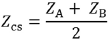
For our case, group sizes are equal. Hence, the mean value of these two centroids is the cutoff score. After that the discriminant function value of each sample is compared with the cutoff score. If its value is greater than cutoff score, then the corresponding sample will be classified as diseased else nondiseased.
►Fig. 1 shows the discriminant scores of all 240 subjects and the respective difference of each subject from their group centroid value. We have two groups in our study, that is, diseased and nondiseased. Hence, we have two centroid values that belong to the two groups.
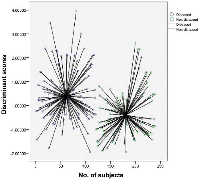
- Scatterplot of discriminant scores of each subject along with their distance from centroid value.
►Fig. 2 shows the discriminant scores of 240 subjects. The centroid value for diseased is 0.407, whereas for nondiseased, it is −0.407. So, the cutoff score will be zero in this case. Hence, the cutoff values above zero are classified as diseased and values below zero are classified as nondiseased.

- Scatterplot of discriminant scores of each subject.
Predictive accuracy of the model: The predictive accuracy of the discriminant function is measured by hit ratio, which is obtained from the classification table. The hit ratio is then compared with the maximum chance criterion that is simply the percentage correctly classified, if all observations were placed in the group with greatest probability of occurrence. Hence, it is the percentage that could be correctly classified by chance without help of discriminant functions. For equal size of groups, the maximum chance criterion is 50%. So, if the model predictive accuracy exceeds the maximum chance criterion, then we can say that our model is valid.
Now we look on the predictive accuracy of models with all four predictive variables as well as excluding X3 variable.
►Table 6 shows that 62.9% of respondents were correctly classified into diseased or nondiseased groups. Nondiseased groups were classified with slightly better accuracy (66.7%) than diseased (59.2%). Cross-validation of the results was performed that found similar to original classification results.
| Original classification | Predicted group membership | Total | |
|---|---|---|---|
| Diseased (%) | Nondiseased (%) | ||
| Diseased | 71 (59.2) | 49 (40.8) | 120 (100) |
| Nondiseased | 40 (33.3) | 80 (66.7) | 120 (100) |
Here, we will discuss relevance of excluding a predictor variable that has nonsignificant mean difference among groups. In our data set X3 as predictor variable has nonsignificant differences between means of diseased and nondiseased groups (►Table 2). Hence, X3 has not considered as a good variable to discriminate between diseased and nondiseased groups.
To create the discriminant equation, unstandardized coefficients (b) have been calculated for all the three predictors after excluding X3.
The discriminant equation as follows:
D2 = (0.019 × X1) + (0.007 × X2) + (0.026 × X4) − 7.489
►Table 7 shows that after excluding X3, predictive accuracy of the model was found to be 67.1%, that is, 67.1% of the respondents were correctly classified into diseased or nondiseased groups. Nondiseased groups were classified with slightly better accuracy (68.3%) than diseased (65.8%).
| Original classification | Predicted group membership | Total | |
|---|---|---|---|
| Diseased (%) | Nondiseased (%) | ||
| Diseased | 79 (65.8) | 41 (34.2) | 120 (100) |
| Nondiseased | 38 (31.7) | 82 (68.3) | 120 (100) |
In both the cases by taking all four variables and excluding variable X3, the calculated model predictive accuracy was found to be 62.9 and 67.1%, respectively. In this case, the maximum chance criterion is 50% that is lower than the model predictive accuracy; hence, both the discriminant models are valid.
Here, we can see that predictive accuracy of the model including all four variables and excluding X3 was increased from 62.9 to 67.1%. So, including a variable with nonsignificant mean differences among groups will compromise the predictive accuracy of the model. Hence, it is suggested to use only those variables in the prediction model having significant mean difference among groups.
Relative Efficiency of DA with Respect to Other Popular Classification Algorithms
All available regression and classification algorithms are supervised learning algorithms. Both the types of algorithms are used for prediction purposes and to utilize the labelled datasets. However, the main difference lies in how they are used for different machine learning problems and their robustness and efficiency. In general, regression algorithms are used to predict the continuous values such as price, salary, and age, whereas classification methods deal with the problem of prediction or classification of the discrete values such as male or female, true or false, etc. In regression, the motive is to find the best fit line, which can predict the output more accurately. In classification, the investigators try to find the decision boundary, which can divide the dataset into different classes. We can further divide the regression-based algorithms into linear and nonlinear regression. The classification problems can also be divided on the basis of whether to use binary classifier or multiclass classifier. The next section is going to present a brief idea about some of the notable classification algorithms (logistic regression, traditional or parametric discrimination methods, tree-based classification methods) together with their suitability, merits, and demerits.
One of the most renowned algorithms is presented by logistic regression, which is much like the linear regression except the way they are used. Linear regression solves regression problems, whereas logistic regression is utilized to deal with the classification problems. Logistic regression (LR) is based on maximum likelihood estimation that estimates probability of group membership and their conditional probabilities. In logistic regression, categorical variables can be used as independent variables while making predictions. The primary merits of logistic regression are that the method is not so exigent to the level of the scale and the form of the distribution in predictors, there is no requirement about the within-group covariance matrices of the predictors, the groups may have quite different sizes, and most importantly the method is not so sensitive to outliers. The other widely used but relatively older classification method is DA that is based on least squares estimation. It is too equivalent to linear regression with binary predictand and estimates probability where the predictand is viewed as binned continuous variable (the discriminant), and it utilizes classificatory device (such as naive Bayes) that requires both conditional and marginal information. LDA, however, needs certain stringent assumptions unlike logistic regression. LDA requires predictors desirably in the interval level with multivariate normal distribution, the within-group covariance matrices should be identical in population, the groups should have similar size. In spite of being quite sensitive to outliers, when all its requirements are met, often LDA is less overfitting, and it performs better than the more robust logistic regression in terms of higher asymptotic relative efficiency.[7] Efron's work also demonstrated that the Bayes prediction of the LDA's posterior class membership probability follows a logistic curve as well. The work of Harrell and Lee showed that the huge increase in relative efficiency of LDA mostly happened in asymptotic cases where the absolute error is practically negligible anyways.[8] There are certain exceptions, like in case of dealing with high dimensional small sample size situations, the LDA still seems superior despite both the assumptions of multivariate normality and the equal covariance matrix assumptions are not met.[9] It is also recommended that the stringent assumptions for LDA are only needed to prove optimality and even if they are not met, the procedure can still be a good heuristic algorithm.[10] LR turns out to be more favorable when the investigator is not dealing with classification problems at all as LR can easily be suitable for the data where the reference has intermediate levels of class membership. On the other hand, linear and/or QDA is preferred to solve normal classification problems.
Apart from the above-mentioned methods, we have tree-based discrimination methods that can take care of both classification and discrimination problems by using decision trees to represent the classification rules. The primary motive of tree-based methods is to divide the dataset into segments, in a recursive manner, such that the resulting subgroups become as homogeneous as possible with respect to the categorical response variable. However, problem arises when cases with a number of measurements (variables) are taken from them. Traditionally, in such circumstances involving two or more groups or populations, investigators prefer to rely on parametric discrimination methods, namely, linear and QDA, as well as the well-known nonparametric kernel density estimation and Kth nearest neighbor rules. As we compare the performance of two traditional discrimination methods, linear and QDA, with two tree-based methods, classification and regression trees (CART) and fast algorithm for classification trees (FACT), using simulated continuous explanatory data and cross-validation error rates, the results often show that the linear and/or QDA should be preferred for normal, less complex data, and parallel classification problems, while CART is best suited for lognormal, highly complex data and sequential classification problems. More precisely, simulation studies using categorical explanatory data also show LDA to work best for parallel problems and CART for sequential problems. CART is said to be preferred for smaller sample sizes a well. FACT is found to perform poorly for both continuous and categorical data.[11]
Detailed Computational Steps Using R Packages
R packages “MASS”, “mda”, “klaR” are essentially used to deal with five types of DA techniques, namely linear, quadratic, mixture, flexible, and regularized discriminant analysis (RDA). The first two comes under “MASS” package; mixture and flexible discriminant analysis (FDA) are done under “mda” package. The RDA is handled by “klaR” package. The entire data analysis process can be divided into a number of tasks, which remain same in all types of DA techniques. First task is to load some necessary packages like “tidyverse” and “caret” for easy data manipulation, visualization, and easy machine learning workflow, respectively. The next task is very essential and it is called the data preparation task. This task can again be divided into two major steps, first the dataset is split into training and test set with admissible proportions, and then we normalize the data by estimating the preprocessing parameters and transforming both the training and test sets by means of using the estimated parameters. The third task is the most critical one in the sense that it requires the investigator to decide which of the above five discriminating techniques should be used based on checking for the assumptions for each of them. For example, before performing LDA, the investigator considers inspecting the univariate distributions of each variable and makes sure that they are normally distributed. If not, the investigator can transform them using log and root for exponential distributions and Box-Cox for skewed distributions. The investigator then removes outliers from the data and standardizes the variables to make their scale comparable. QDA is little bit more flexible than LDA as it disregards the equality of variance/covariance assumption. In other words, for QDA the covariance matrix can be different for each class. LDA is preferred when the investigator has a small training set. In contrast, QDA is recommended if the training set is very large, so that the variance of the classifier is not a subject of concern, or if the assumption of a common covariance matrix for the K classes can clearly not be maintained.[12] For mixed discriminant analysis (MDA), there are classes and each of them is assumed to be a Gaussian mixture of subclasses. In this setup, each data point has a probability of belonging to each class, and equality of covariance matrix, among classes, is still the assumption that should be validated. FDA becomes useful to model multivariate nonnormality or nonlinear relationships among variables within each group, allowing for a more accurate classification. The last one, that is the RDA is considered to be a kind of a tradeoff between LDA and QDA, as it shrinks the separate covariances of QDA toward a common covariance as in LDA and thus builds a classification rule by regularizing the group covariance matrices allowing a more robust model against multicollinearity in the data.[13] This might be very useful for a large multivariate data set containing highly correlated predictors.
Once the method is decided, the next tasks are same for all the above-mentioned methods. The investigator fits the model on the transformed trained dataset by using the respective functions [lda(), qda(), mda(), fda() and rda()] under the appropriate packages. lda(), for example, returns three outputs: prior probabilities of groups, group means or group center of gravity, and coefficients of linear discriminants (shows the linear combination of predictor variables that are used to form the LDA decision rule). In all the above methods, predict() function is used on the transformed test dataset in order to make prediction. predict() function returns three elements, class (predicted classes of observations), posterior (a matrix whose columns are the groups, rows are the individuals and values are the posterior probability that the corresponding observation belongs to the group) and x (contains the linear discriminants).
The last task is to check the model accuracy by means of using the function mean(). This function returns a value between 0(0% accuracy) and 1(100% accuracy) including both the limits. The investigator can further visualize the decision boundaries using different clustering packages (“mclust”), tools and functions [ggplot() under “ggplot2”] for generating plots and thus can present more insightful details that can help evaluating model performance.
Conclusion
Discriminant function analysis is a statistical tool that is used for predicting the accuracy of a classification system or predictor variables. It has various applications in public health and clinical field as it can be used for validating the newly developed classification system or predictors that can categorize samples into different groups. This article describes the various assumptions, analysis, and interpretation of the output tables of DA in simplified form by taking clinical example for the better understanding.
Conflict of Interest
None declared.
Funding
None.
References
- Accessed March 3, 2022 from http://www.econ.upf.edu/~satorra/AnalisiMultivariant/Chapter25DiscriminantAnalysis.pdf
- How to measure habitat: a statistical perspective. US Forest Service General Technical Report RM. 1981;87:53-57.
- [Google Scholar]
- Discriminant functions when covariances are unequal and sample sizes are moderate. Biometrics. 1977;33:479-484.
- [CrossRef] [Google Scholar]
- Assessment of sampling stability in ecological applications of discriminant analysis. Ecology. 1988;69(04):1275-1285.
- [CrossRef] [Google Scholar]
- Gallstone disease and quantitative analysis of independent biochemical parameters: study in a tertiary care hospital of India. J Lab Physicians. 2018;10(04):448-452.
- [CrossRef] [PubMed] [Google Scholar]
- The efficiency of logistic regression compared to normal discriminant analysis. J Am Stat Assoc. 1975;70:892-898.
- [CrossRef] [Google Scholar]
- A comparison of the discrimination of discriminant analysis and logistic regression under multivariate normality, Biostatistics: Statistics in Biomedical, Public Health and Environmental Sciences. North-Holland, New York: United States; 1985. p. :333-343.
- [Google Scholar]
- Raman spectroscopic grading of astrocytoma tissues: using soft reference information. Anal Bioanal Chem. 2011;400(09):2801-2816.
- [CrossRef] [PubMed] [Google Scholar]
- The Elements of Statistical Learning; Data mining, Inference and Prediction. New York: Springer Verlag; 2009.
- [CrossRef] [Google Scholar]
- “A comparison of tree-based and traditional classification methods: a thesis presented in partial fulfilment of the requirements for the degree of PhD in Statistics at Massey University.”. PhD diss. Massey University; 1994.
- [Google Scholar]
- Regularized discriminant analysis. J Am Statistic Assoc. 1989;84(405):165-75.
- [CrossRef] [Google Scholar]